
Python and Momentum Trading Strategy (Backtest, Rules, Code, Setup Overview)
There are many factors that quants and algorithmic traders use when they develop trading strategies. Some of them are value, quality, size and, the one we will be backtesting today, momentum.
Momentum is an investing factor that aims to benefit from the ongoing trend of a stock or asset. A stock that has been rising is said to have positive momentum while a stock that has been crashing is said to have negative momentum. We show you how to code such a strategy using Python.
In this article, we are going to show you how to backtest a momentum trading strategy in Python: from downloading the data and calculating momentum to backtesting the strategy and plotting the results.
The first step to backtest any trading strategy is to gather the necessary data. In this case we are going to download the historical data using the library yfinance. If you want to know more about how to download not only historical stock prices but also fundamental data from the Yahoo Finance website check out these two posts:
- How To Download Data For Your Trading Strategy From Yahoo!Finance With Python
- How To Build A Trading Strategy From FRED Data In Python (Strategy, Backtest, Rules)
For the purpose of this backtest, we will also use the libraries pandas, numpy and matplotlib.pyplot.
Related reading:
- A comprehensive list of stock market trading systems
- Python Trading Strategy Backtesting – How To Do It (Plenty of examples with code and images)
Downloading historical data
Regarding the strategy we are going to backtest today, we are going to be using the select sectors SPDR ETFs. The ticker symbols are:
- XLK: Technology
- XLY: Consumer discretionary
- XLP: Consumer staples
- XLU: Utilities
- XLI: Industrials
- XLE: Energy
- XLF: Financials
- XLV: Healthcare
- XLC: Communications
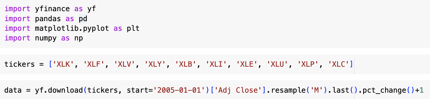
With this in mind, all we need to do is create a list with all the tickers symbols, define a variable(data), and use the yf.download() function to download the data. Take into account we will only use the adjusted close prices. You should always use adjusted data to make sure you include dividends. Dividends make up a large part of total returns for a lot of assets.
The strategy will rebalance the portfolio monthly so we will use the .resample(‘M’).last() function to keep just the last monthly closing price of the ETF. Lastly, we use the pct_change() function and add 1 to get the percentage change from the previous month
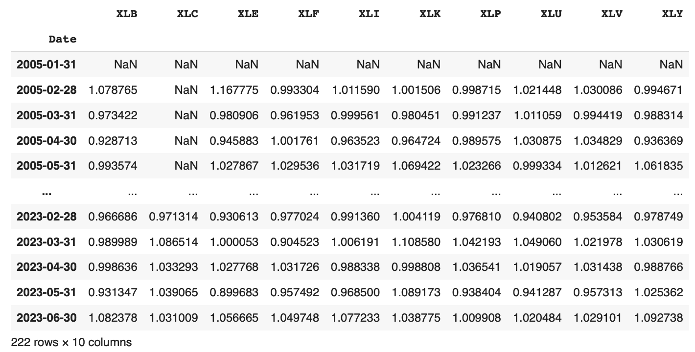
And here is the output if we print data:

We now have the monthly change of every ETF going back to 2005!
Calculating the momentum factor
There are many ways to measure the momentum of a stock or ETF. In this backtest, we will define it as the rolling past 9 month performance of the ETF.
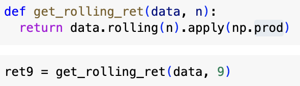
To calculate it we will create a function called get_rolling_ret() which receives two inputs: the data and the number of months to calculate the past performance.
Then we will define a new variable(ret9) and run this function using as input the variable data and 9 (because we want the performance of the last 9 months).
The results will be a dataframe of the past 9 month performance of each ETF in every month:
The trading rules – momentum strategy in Python
The trading rules of the strategy are the following:
Trading Rules
[am4show have=’p2;p3;p58;p59;p130;p138;’ user_error=’Premium Post Access’ guest_error=’Premium Posts’]
Every month we measure the momentum of each ETF and buy and hold the top 3 with the highest momentum the prior month. The strategy is rebalanced monthly.
So for example, if XLE, XLK, and XLI had the highest 9 month performance of all the ETFs in March, we will buy and hold them in April. At the end of April we will re-evaluate momentum again, and determine which 3 ETFs should we hold in May.
[/am4show]
Calculating the returns of the strategy
In order to code the above trading rules, we are going to create two functions. The first one is get_top(). The input of the function is a date. What it does is return the 3 ETFs that have the best 9 mo